Here I write about GMMs because it's a method of clustering that serves as a basis for more advanced concepts.
In [1]:
In [1]:
import matplotlib.pyplot as plt
import numpy as np
from scipy import stats
import seaborn as sns
import pandas as pd
from math import sqrt, log, exp, pi
from random import uniform
%matplotlib inline
In [2]:
#read our dataset
df = pd.read_csv("data/bimodal_example.csv")
data = df.x
data.head()
Out[2]:
Here, the problem is unsupervised, and it is about clustering.
A universally used generative unsupervised clustering method is Gaussian Mixture Model (GMM), which is also known as "EM Clustering."
These are 2 types of clustering:
$$p(x | \theta) = \mathcal N(x \ | \ \mu, \sigma^2)$$
A universally used generative unsupervised clustering method is Gaussian Mixture Model (GMM), which is also known as "EM Clustering."
These are 2 types of clustering:
- Hard Clustering: for each data point assign a cluster
- Soft Clustering: for each data point assign a probability distribution over clusters
Fitting a single gaussian
In a one-dimensional case, there's this probability distribution that might represent the whole dataset.$$p(x | \theta) = \mathcal N(x \ | \ \mu, \sigma^2)$$
In [3]:
gfit_mean = np.mean(data)
gfit_sigma = np.std(data)

x = np.linspace(-6, 8, 200)
g_single = stats.norm(gfit_mean, gfit_sigma).pdf(x)
sns.distplot(data, bins=20, kde=False, norm_hist=True)
plt.plot(x, g_single, label='single gaussian')
plt.legend();
Two Gaussians would represent the data better.
In [4]:
sample_gauss_1 = np.random.multivariate_normal([0, 0], [[1, 0], [0, 100]], 100)
sample_gauss_3 = np.random.multivariate_normal([10, 10], [[10, 0], [0, 10]], 100)

data_2d = np.vstack((sample_gauss_1, sample_gauss_3))
plt.scatter(data_2d[:,0], data_2d[:,1])
Out[4]:
In [5]:
gfit_mean = (np.mean(data_2d[:,0]), np.mean(data_2d[:,1]))
gfit_sigma = np.cov(data_2d.T)

ngrid = 10
xlim = (-15, 25)
ylim = (-15, 25)
x = np.linspace(xlim[0], xlim[1], ngrid, endpoint=True)
y = np.linspace(ylim[0], ylim[1], ngrid, endpoint=True)
X, Y = np.meshgrid(x, y)
xy = np.vstack([X.ravel(), Y.ravel()]).T

z = np.array([stats.multivariate_normal.pdf(xy_elem, gfit_mean, gfit_sigma) for xy_elem in xy])
z = z.reshape((ngrid, ngrid))
plt.scatter(data_2d[:,0], data_2d[:,1])
plt.contour(x, y, z, cmap=plt.cm.jet)
Out[5]:
But there is a more approximate Gaussian that can be used to generate the data: a mixture of Gaussians. In the last example, 2 Gaussians would do the trick.
Defining a model
We need two Normal distributions $\mathcal N(\mu_1, \sigma_1^2)$ and $\mathcal N(\mu_2, \sigma_2^2)$.Hence, there are 5 parameters: 4 of them are from Normal distributions, and 1 more for the probability of choosing one of them.
Let $\psi$ be the probability that the data comes from the first Normal, the parameter in this model is $\theta = (\psi, \mu_1, \sigma_1^2, \mu_2, \sigma_2^2)$.
This is the probability of the occurrence of a data point
$$ p(x | \theta) = \psi \mathcal N(x | \mu_1, \sigma_1^2) + (1 - \psi) \mathcal N (x | \mu_2, \sigma_2^2) $$
Optimization problem
Max. likelihood$$ \begin{align} \max_\theta &\prod_{i=1}^N p(x_i|\theta) \\ \max_\theta &\prod_{i=1}^N \psi \mathcal N(x_i | \mu_1, \sigma_1^2) + (1 - \psi) \mathcal N (x_i | \mu_2, \sigma_2^2) \end{align} $$
Introducing a latent variable (LV)
Each data point was generated by using some LV "z" that will take 2 values: 1 and 2.Expectation Maximization (EM) can be used to estimate $\theta$
EM Algorithm for GMM
Continuing with the mixture of normals model as our example, we can apply the EM algorithm to estimate $\theta = \{\mu, \sigma, \psi\}$.This was copied from https://github.com/fonnesbeck/Bios8366/ Initiazlize all parameters $\theta_0 = \{\mu_0, \sigma_0, \psi_0\}$
Repeat until convergence:
- E-step: guess the values of $\{z_i\}$
$$P(z_i = j | x_i) = \frac{P(x_i | z_i=j) P(z_i=j)}{\sum_{l=1}^k P(x_i | z_i=l) P(z_i=l)}$$
$P(z_i=j|\theta) = \psi_j$
$P(x|z_i=j, \theta) = \mathcal N (x | \mu_j, \sigma_j)$
$\theta$ has been dropped for notational convenience.
- M-step: update estimates of parameters $\theta$
In [6]:
class Gaussian:
    "Model univariate Gaussian"

    def __init__(self, mu, sigma):
        self.mu = mu
        self.sigma = sigma

    def pdf(self, datum):
        u = (datum - self.mu) / abs(self.sigma)
        y = (1 / (sqrt(2 * pi) * abs(self.sigma))) * exp(-u * u / 2)
        return y

    def __repr__(self):
        return 'Gaussian({0:.03}, {1:.03})'.format(self.mu, self.sigma)

class GaussianMixture:
    "Model mixture of two univariate Gaussians and their EM estimation"

    def __init__(self, data, mu1_ini, sigma1_ini, mu2_ini, sigma2_ini, psi=.5):
        self.data = data
        self.one = Gaussian(mu1_ini, sigma1_ini)
        self.two = Gaussian(mu2_ini, sigma2_ini)
        self.psi = psi

    def Estep(self):
        self.loglike = 0.
        for x in self.data:
            wp1 = self.one.pdf(x) * self.psi
            wp2 = self.two.pdf(x) * (1. - self.psi)
            den = wp1 + wp2
            # normalize
            wp1 /= den
            wp2 /= den
            # add into loglike
            self.loglike += log(wp1 + wp2)
            yield(wp1, wp2)

    def Mstep(self, weights):
        # compute denominators
        (left, right) = zip(*weights)
        one_den = sum(left)
        two_den = sum(right)
        # compute new means
        self.one.mu = sum(w * d / one_den for (w, d) in zip(left, data))
        self.two.mu = sum(w * d / two_den for (w, d) in zip(right, data))
        # compute new sigmas
        self.one.sigma = sqrt(sum(w * ((d - self.one.mu) ** 2)
                                  for (w, d) in zip(left, data)) / one_den)
        self.two.sigma = sqrt(sum(w * ((d - self.two.mu) ** 2)
                                  for (w, d) in zip(right, data)) / two_den)
        # compute new psi
        self.psi = one_den / len(data)

    def fit(self, n_iterations, verbose=True):
        best_loglike = float('-inf')

        for i in range(n_iterations):
            if verbose:
                print('{0} loglike: {1}, {2}'.format(i, best_loglike, self))

            self.Mstep(self.Estep())

            if self.loglike > best_loglike:
                best_loglike = self.loglike

    def pdf(self, x):
        return (self.psi)*self.one.pdf(x) + (1-self.psi)*self.two.pdf(x)

    def __str__(self):
        return 'GaussianMixture: {0}, {1}, psi={2:.03})'.format(self.one,
                                                        self.two,
                                                        self.psi)
In [7]:
n_iterations = 100
GMM = GaussianMixture(data, -5., 10., 5., 10.)
GMM.fit(n_iterations)
In [8]:
x = np.linspace(-6, 8, 200)
sns.distplot(data, bins=20, kde=False, norm_hist=True)
g_both = [GMM.pdf(e) for e in x]
plt.plot(x, g_both, label='gaussian mixture');
plt.legend();
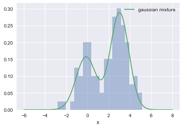
This can be seen as 2 clusters.
After the posterior of a latent variable $z$ was computed $P(z_i = j | x_i, \theta)$, a better fit was found.
After the posterior of a latent variable $z$ was computed $P(z_i = j | x_i, \theta)$, a better fit was found.
