Some stuff learned from I Heart Stats: Learning to Love Statistics about Inferential Statistics.

My null hypothesis will be that there's no relationship (the relationship is zero).
When you "Test a Null Hypothesis", you have to show that the relationship is not zero or at least show that it's not zero with a certain level of certainty.
An Example about a class of 100 students, where there are 30 men, 70 women.

We got those expected values from the observed values. The expected values of each cell are computed like this, $12 = (30*40) / 100$
We use the Chi-Square test because we need to find out whether those numbers really mean something statistically.
$$\chi^2 = \sum \frac{(f_o - f_e)^2}{f_e}$$$$f_o = \text{Observed Frequency}$$$$f_e = \text{Expected Frequency}$$

Then we calculate the Chi-Square
$$\chi^2 = 12.7$$
To use this test, the independent variable has to be "Nominal", and the dependent variable has to be "Interval" or "Ratio".
For example, we have the following information from two groups, the number of hair products used by men and women. The independent variable is gender (Nominal Level) and the dependant variable is number of hair products (Ratio Level).
$$\overline{X_1} = 3.5, N_1 = 12, S_1 = 1.80$$$$\overline{X_2} = 2.9, N_2 = 10, S_2 = 1.51$$
And we define the following:
$$\overline{X_1} - \overline{X_2} = 0.6$$
But I wanna see whether or not they are significantly different, taking into account their $N$ and $S$. Then I use the "T-test".
$$t = \frac{\overline{X_1} - \overline{X_2}}{\hat{\sigma}_{\overline{X_1} - \overline{X_2}}}$$$$ \hat{\sigma}_{\overline{X_1} - \overline{X_2}} = \sqrt{\frac{N_1 S_1^2 + N_2 S_2^2}{N_1 + N_2 - 2}} \sqrt{\frac{N_1 + N_2}{N_1 N_2}}$$
$\hat{\sigma}_{\overline{X_1} - \overline{X_2}}$ is the estimated standard error of the mean for the population.
First, I mention two important concepts.

In many, many statistical situations, we use what's called
Significance Level: Probability of incorrectly rejecting $H_0$.
It's very common to use a "0.05 significance level". Then the chance that we're wrong is 0.05 or 5%. This means we're finding something that's outside of the middle segment of the distribution. We use this value to do Statistical Significance Testing of a statistic measured from the data.
- Population: Every observed element.
- Sample: Subset of cases or individuals of the population.
Normal Distribution
- Given the mean $\mu$ and the standard deviation $\sigma$. We find that a certain percentage of the cases are within certain standard deviations away from the mean.
- In some cases, we could say that 68% of the individuals are between one standard deviation unit. This means between one standard deviation below and above the mean. The same for the region of 95% and the one of 99.7%.
In many, many statistical situations, we use what's called
Significance Level: Probability of incorrectly rejecting $H_0$.
It's very common to use a "0.05 significance level". Then the chance that we're wrong is 0.05 or 5%. This means we're finding something that's outside of the middle segment of the distribution. We use this value to do Statistical Significance Testing of a statistic measured from the data.
- Statistical Significance plays a pivotal role in statistical hypothesis testing, where it is used to determine whether a Null Hypothesis should be rejected or retained.
The Null Hypothesis
For example, if I have an hypothesis that there's a relationship between two variables (this means that the relationship is not zero).My null hypothesis will be that there's no relationship (the relationship is zero).
When you "Test a Null Hypothesis", you have to show that the relationship is not zero or at least show that it's not zero with a certain level of certainty.
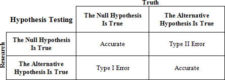
There are two types of Hypothesis. For example, if I think that education is related to income, then that's what my Research or Alternative Hypothesis ($H_0$) is. It's got a relationship with another thing that's really important here, that's called the Null Hypothesis ($H_1$).
There's also:
But if it's not, we fail to reject (accept) the Null Hypothesis and reject the Research Hypothesis. Also, we say that the statistic is actually significant and it's meaningful beyond just random chance.
There's also:
- One-Tailed Research Hypothesis: For example, education is related to income
- Two-Tailed Research Hypothesis: For example, education drives up income
- The sample taken is representative of the population
- The way you are measuring them is valid
- Assume that the variables under investigation have a Normal Distribution
- Find a Dependant and Independent variable
- Set a Hypothesis, there's the one that's called the "Research Hypothesis or Alternative Hypothesis" and the "Null Hypothesis"
- Pick the test in a basis of the level of measurement
- Pick a Significance level (0.05)
- Find the Critical Value (so that we can compare a Calculated Value with this value).
- Make a decision: We can reject the null hypothesis or not
But if it's not, we fail to reject (accept) the Null Hypothesis and reject the Research Hypothesis. Also, we say that the statistic is actually significant and it's meaningful beyond just random chance.
- Find the meaning of the results
Statistical Test - Chi Square
Pairs of variables with which we can use the Chi-Square test: (nominal, nominal), (nominal, ordinal), (ordinal, nominal), (ordinal, ordinal)An Example about a class of 100 students, where there are 30 men, 70 women.
- Research Hypothesis: There is a relationship between gender and cheating.
- Null Hypothesis: There is no difference between men and women in the amount of cheating they did.
We got those expected values from the observed values. The expected values of each cell are computed like this, $12 = (30*40) / 100$
We use the Chi-Square test because we need to find out whether those numbers really mean something statistically.
$$\chi^2 = \sum \frac{(f_o - f_e)^2}{f_e}$$$$f_o = \text{Observed Frequency}$$$$f_e = \text{Expected Frequency}$$
Then we calculate the Chi-Square
$$\chi^2 = 12.7$$
Degrees of Freedom (df): The previous table has just 1 degree of freedom. This means that there's only one cell I need, so that the other cells are filled easily.

We can reject or fail to reject (or accept) the Null Hypothesis according to a Critical Value that's obtained from a predefined "Chi-Square Table".

And because we have a significance value of $0.05$. The Critical Value is $3.841$.
Then comparing
$$12.7 > 3.841$$
We accept the notion that there actually is a relationship between the variables. We reject the null hypothesis. Which means there is a relationship between gender and cheating.
We can reject or fail to reject (or accept) the Null Hypothesis according to a Critical Value that's obtained from a predefined "Chi-Square Table".
And because we have a significance value of $0.05$. The Critical Value is $3.841$.
Then comparing
$$12.7 > 3.841$$
We accept the notion that there actually is a relationship between the variables. We reject the null hypothesis. Which means there is a relationship between gender and cheating.
Now here's an example of working with Ordinal Data about what to do first when washing your teeth. We have some responses from people.

Then the table of observed values will look like.

Then the table of observed values will look like.
Statistical Test - T-Test
This test is used to compare means when we have two groups in the independent variable. If we have more than two, we should use ANOVA, which is the next one. Also, it doesn't matter which variable is first, $t$ can have a negative sign.To use this test, the independent variable has to be "Nominal", and the dependent variable has to be "Interval" or "Ratio".
For example, we have the following information from two groups, the number of hair products used by men and women. The independent variable is gender (Nominal Level) and the dependant variable is number of hair products (Ratio Level).
$$\overline{X_1} = 3.5, N_1 = 12, S_1 = 1.80$$$$\overline{X_2} = 2.9, N_2 = 10, S_2 = 1.51$$
And we define the following:
- Research Hypothesis: Women use a significantly higher number of hair products than men do.
- Null Hypothesis: There is no significant difference in the number of hair products used by gender.
$$\overline{X_1} - \overline{X_2} = 0.6$$
But I wanna see whether or not they are significantly different, taking into account their $N$ and $S$. Then I use the "T-test".
$$t = \frac{\overline{X_1} - \overline{X_2}}{\hat{\sigma}_{\overline{X_1} - \overline{X_2}}}$$$$ \hat{\sigma}_{\overline{X_1} - \overline{X_2}} = \sqrt{\frac{N_1 S_1^2 + N_2 S_2^2}{N_1 + N_2 - 2}} \sqrt{\frac{N_1 + N_2}{N_1 N_2}}$$
$\hat{\sigma}_{\overline{X_1} - \overline{X_2}}$ is the estimated standard error of the mean for the population.
Returning to the example we get $t = 0.811$
Then again we need to know a critical value, which is of course taken from a predefined table:

And we need to know the following to get this value.
$$0.811 < 1.725$$
We say that we've failed to reject the Null Hypothesis, which means that there is no significant difference in the number of hair products used by gender.
And because of the $0.05$ or $5\%$ significance level, we can state that there's $95$ percent of certainty that there is no significant difference.
Next post: http://relguzman.blogspot.com/2015/07/reviewing-inferential-statistics-part-2.html
Then again we need to know a critical value, which is of course taken from a predefined table:
And we need to know the following to get this value.
- Significance Level
We define a significance level of 0.05.
- Degrees of Freedom
$$
\begin{align}
df& = (N_1 - 1) + (N_2 - 1)\\
df& = 20
\end{align}
$$
- Is it a One or Two Tailed Test?
And in this case, it's a One-Tailed Test (it will regularly be One-Tailed)
Now we can get the Critical Value for this test. It will be $1.725$. Then we compare both values.
We say that we've failed to reject the Null Hypothesis, which means that there is no significant difference in the number of hair products used by gender.
And because of the $0.05$ or $5\%$ significance level, we can state that there's $95$ percent of certainty that there is no significant difference.
Next post: http://relguzman.blogspot.com/2015/07/reviewing-inferential-statistics-part-2.html